Hosein Mohimani Curriculum Vitae
Research
Discovering Antibiotics from Omics Big Data
Ever since Alexander Fleming accidentally discovered penicillin, there has been a constant warfare between the pharmaceutical companies and antibiotics resistance bacteria. During the last seven decades, the pharmaceutical companies have been developing novel antibiotics, and the microbes have been developing resistance against them. The pharmaceutical firms have been winning till very recently, but not anymore! That is the reason why in 2015, President Obama announced a national strategy to combat bacterial resistance. And its not surprising that last year the Nobel Prize in medicine went to three researchers working on antibiotic and antimalarial compounds.
Challenge of Antibiotic Sequencing
The way research is conducted in the field of antibiotics discovery has not changed much in the last 50 years. According to Thomas Frieden, the director of the Centers for Disease Control and Prevention, “The medicine cabinet is empty for some patients. It is the end of the road for antibiotics unless we act urgently.” We believe the main bottleneck in antibiotics discovery is the lack of computational techniques to streamline the discovery process. In this documents I discuss several open problems in computational antibiotic discovery for computer scientists and statisticians. Before getting to the open problems, I need to give a brief background.
Automated antibiotics discovery relies on the techniques from genomics, proteomics and metabolomics (Figure 1). Genomics studies focus on the static DNA sequences of an organisms, while proteomics and metabolomics focus on the dynamic protein and metabolite products of the genome. While the computational techniques in genomics and proteomics have been extensively studies in the last two decades, metabolomics is a novel field that has barely been touched by computer scientists and statisticians.
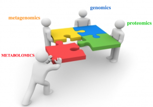
Figure 1. In addition to more traditional techniques from genomics, proteomics and metagenomics, antibiotic discovery relies on techniques from metabolomics.
The Central Dogma of Biology
The Central Dogma of Biology states that the DNA is transcribed to RNA by RNA-polymerase, and the RNA is translated to proteins by ribosome. In 1958, Edward Tatum made an extra-ordinary observation. When Tatum inhibited the ribosome in a microbe called Bacillus brevis, the microbe continued to produce a short peptide. But how can a microbe produce peptides without any ribosome? It turned out that the central dogma was not the only pathway for production of peptides. There is a large family of peptides called non-ribosomal peptides (NRPs) that can be produced with no ribosome.
Non-Ribosomal Peptides
NRPs include some of the most effective antibiotics in the history of medicine, including Penicillin. But how these peptides are synthesized? It turned out that NRPs are produced by gigantic modular enzymes called non-ribosomal peptide synthetase (NRPS).
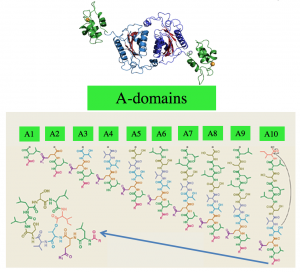
a)
b)
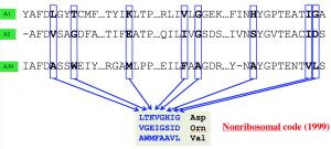
Figure 2. (a) Each A-domain incorporates a single amino acid into the backbone of the NRP. The last domain usually cyclize the NRP. (b) The NRP code postulates that a specific substring of length 8 of the A-domain defines the amino acid loaded by the domain.
NRP code
Production of a NRP of length 10 amino acids requires an NRPS with 10 modules (called A-domains) and a length of roughly 100,000 amino acids. NRPs are so vital for microbes that some of the microorganisms assign 20-30% of their genome just for production of these peptides.
All A-domains are evolutionarily related and its possible to align their sequences. In 1999 Mohammed Marahiel discovered that very similar to the genetic code that translates each three nucleic bases to a protein, there is a non-ribosomal code that governs what amino acid each A-domains incorporate into the backbone of NRP. The NRP code postulates that a specific substring of length 8 of the A-domain defines the amino acid loaded by the domain. (Figure 2). In 2005, supervised learning based tools were developed to predict the structure of an NRP from NRPS.
The Bottleneck of supervised learning
The supervised learning methods for mining antibiotics genes have contributed greatly to the field during the last decade. However, these methods suffer from the lack of labelled training data. As a result, the top predictions of supervised learning methods is often incorrect, specially for exotic amino acids for which we do not have a lot of training data (Figure 3). It is possible to use metabolomics data to correct errors from these supervised learning techniques.
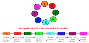
Figure 3. Top three supervised learning predictions for A-domains of a NRP with length 8. The top prediction is incorrect for four out of eight residues.
The traditional approach to antibiotics discovery
The traditional approach to antibiotics discovery is time consuming and expensive. Moreover, this process often results in rediscovery of known antibiotics, rather than novel ones. Our goal is to bring techniques from computer sciences and statistics to automate the process of natural product discovery.
Metabolomics
The main technologies in metabolomics are mass spectrometry (MS) and nuclear magnetic resonance (NMR). Mass Spectrometry has the advantage of being fast, inexpensive, and it can work on complex samples (taken from environment or host) and very small (picograms) of material, while NMR is very accurate (Figure 4). Our goal is to combine mass spectrometry with genomics to make it accurate.
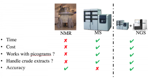
Figure 4. The main technologies in metabolomics are mass spectrometry (MS) and nuclear magnetic resonance (NMR).
Mass Spectrometry
A peptide antibiotic can be modeled as a graph, where each node is an amino acid and each edge is a peptide bond. Mass spectrometry cuts this graph from all possible bridges and 2-cuts, and measure the mass of each connected component from cuts, which is the sum of the masses of all its amino acids. These masses (called mass spectra) are given in no specific order, and we want to identify the masses of all amino acids in peptide antibiotic graph from mass spectra (Figure 5).
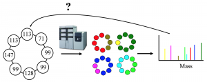
Figure 5. A peptide antibiotic can be modeled as a graph, where each node is an amino acid and each edge is a peptide bond. Mass spectrometry cuts this graph from all possible bridges and 2-cuts, and measure the mass of each connected component, which is the sum of the masses of all its amino acids. These masses (called mass spectra) are given in no specific order, and we want to identify the masses of all amino acids in peptide antibiotic graph from mass spectra.
Relationships to Turnpike problem
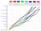
The problem of sequencing peptide from mass spectrometry resembles the classic turnpike and beltway problems in computer sciences. In the turnpike problem, we have a set of exits in a highway, and we are given the pairwise distances between these exits. The goal is to reconstruct the position of exits on the highway from these pairwise distances. To make the problem even more difficult, in real world applications some of the pairwise distances are missing, and we also have noise (Figure 6).
The turnpike problem is shown to be an NP-hard problem in noisy case. Our goal is to use genome mining results as a cheat sheet to solve a special case of the turnpike problem.
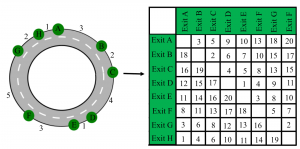
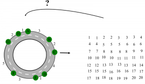
Figure 6. In turnpike problem, we want to reconstruct the consecutive distance of exits in a highway from pairwise distances.
Antibiotics Discovery from complex samples
The first antibiotics penicillin, was accidentally discovered from a rotten melon. Since then, majority of the antibiotics have been discovered from microbes living in environmental natural samples. However, most of the environmental samples are complex, with thousands of microbial strains living together. Metagenomics data collected on these complex samples tell us what microbes are living there, and metabolomics data tells what chemicals these microbes produce. Our goal is to use Big Data from metabolomics and metagenomics to characterize antibiotics from complex samples.
Genomics and Metagenomics Assembly
Genomics and metagenomics reads from next generation sequencing are given as short reads (100 to 300 base pairs) from an alphabet of A, G, C and T. Assembling genomes and metagenomes from billions of overlapping DNA substrings resembles solving puzzles from error-prone pieces. In the error-free case, this problem is equivalent to finding Eulerian path in a giant de bruijn graph (Figure 7).

Figure 7. Assembling genomes and metagenomes from billions of overlapping DNA substrings resembles solving puzzles from error-prone pieces. In the error-free case, this problem is equivalent to finding Eulerian path in a giant de bruijn graph.
Antibiotics Discovery: metabolomics meet metagenomics
Antibiotics discovery by metagenomics and metabolomics starts from collecting environmental and host-associated samples. These samples can be collected from untouched areas of earth (e.g. sponges and lichens in the oceans) or human body sites. Human microbiomes contains microbes that produce antibiotics that are shown to kill human pathogens, and this makes them potential drug candidates.
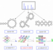
The next step is to collect metagenomics and mass spectrometry data on the samples. Metagenomics data is assembled, and the metagenomics assembly in mined using the supervised learning methods introduced in section NRP code to identify NRP synthetases. During the last decade, there has been extensive research on the questions of “What antibiotics are encoded by these NRP synthetases”, and “What antibiotics are encoded by these mass spectra”. The metabologenomics approach to antibiotics discovery answers both these questions simultaneously by building a bridge between mass spectrometry and metagenomics (Figure 8).
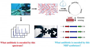
Figure 8. Metabolomics meets metagenomics.
The metabologenomics bridge
Now we have short reads (100-300 base pair reads of A,C,G &T) from metagenomics and mass spectra (vectors of masses), and we want to identify the structures of all antibiotics in these samples (Figure 9). After finding NRP genes, all possible candidate antibiotics structures are constructed from these genes. Note that we can have multiple candidates for each NRP gene due to ambiguity of NRP code. Then, the predicted mass spectra are constructed for each candidate NRP structure by cutting them from all the possible bridges and 2-cuts. Note that this procedure results in of predicted spectra, majority of them corresponding to infeasible antibiotics structures. Then predicted spectra is compared against the mass spectra (billions of spectra) to find similarities and detect feasible antibiotics structures. Because pairwise comparison of datasets of size billion is impractical, we need to come up with more efficient methods for this task, discussed in section Open Problems : Big Data. Moreover, each comparison between the predicted spectra and mass spectra should be done in an error tolerant manner, due to the noise in metabolomics and metagenomics data. This challenge is discussed in section Open Problems : error tolerant matching. Finally, we need to asses the statistical significance of results, which is discussed in Open Problems : statistical validation of the results.
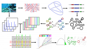
Figure 9. Metabologenomics pipeline
Open Problems
In this section, I propose several open problems in the area of antibiotics discovery by Omics Big Data. These problems are independent and self-contained.
Open Problems : Matching Omics Big Data
In its simplest form, a mass spectrum/predicted spectrum is modeled by a binary vector with 1s at positions where the corresponding mass is present, and 0 when it is absent. Modern mass spectrometers have a mass range of 0-2000Da and accuracy of 0.01Da, resulting in sparse vectors of size 200,000, with roughly 100 ones (Figure 10).
The shared-peak count score of two spectra is defined as their dot product, and the problem of matching metabolomics data to metagenomics data amounts to finding all pairs of vectors from a given set of vectors with dot products higher than a threshold. The brute force approach has a complexity of O(N2) for datasets of size N, making it intractable for billions of spectra.
It turned out that a very similar problem emerged in gene expression for finding genes that are co-expressed under similar conditions, and in document clustering for finding documents that share a lot of words.
Biclustering of a data matrix refers to simultaneous clustering of it rows and columns into sub-matrices of similar behavior and has been applied to gene expression (genes and conditions), marketing (customers and product) and document-word clustering (documents and words).
The goal here is to develop an efficient pipeline for matching billions of mass spectra against billions of predicted spectra.
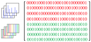
Figure 10. The problem of matching metabolomics data to metagenomics data amounts to finding all pairs of vectors from a given set of vectors with dot products higher than a threshold.
Open Problems : Error Tolerant Matching
Machine learning predictions of antibiotic structure from metagenomes are error-prone, especially for the less studied microbial strains for which smaller training datasets are available. We attempt to error correct metagenomics predictions from metabolomics data. This problem resembles the problem of demodulating digital data from an analog signal corrupted by noise in a communication channel. Since Viterbi decoding provides the optimal solution to the demodulation problem, it can be applied to connecting metabolomics data to metagenomics data while allowing for variations between the two (Figure 11).
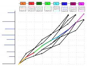
Figure 11. Viterbi decoding provides the optimal solution for error tolerant matching of metabolomics data to metagenomic data
Open Problems : Matching Graphs
In practice, it is impossible to assemble metagenomics short reads into complete microbial genomics. Modern assemblers congregate short reads into assembly graphs. Complex metagenomics samples contain thousands of antibiotics genes each corresponding to a subgraph of the assembly graph. Our goal is to align thousands of graphs to billions of mass spectra. This is a generalization of both multiple sequence alignment, and biclustering (Figure 12).
Open Problems : Statistical validation of results
When searching billions of mass spectra against metagenomes with billions of base pairs, one needs to compute the statistical significance of matches between the metabolomics and metagenomics data, and filter out wrong matches based on the statistical significance (Figure 13). P-value of a match between metabolomics and metagenomics data is defined as the portion of randomly generated data with scores exceeding match score.
The naive Monte Carlo approach is computationally intractable for p-value below 10-6. The problem of computing very small p-value of match scores between metabolomics data and metagenomic data is equivalent to finding the probability of visiting a rare state in a markov chain, and importance sampling based methods can be utilized for solving it.
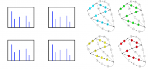
Figure 12. Antibiotics genes are subgraphs of the assembly graph. Each path in an antibiotic gene subgraph corresponds to a feasible antibiotic structure. When linking metabolomics data to metagenomics data, we need to align billions of mass spectra against thousands of antibiotics gene subgraphs.
Open Problems : Learning fragmentation pattern in metabolomics by graphical models
Given a chemical structure, how can we predict its mass spectra? Given a mass spectrum, how can we identify which chemical structure does it correspond to? These are open problems that we are trying to solve using large scale pairs of mass spectra and chemical structures.
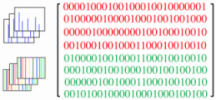
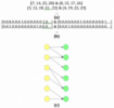
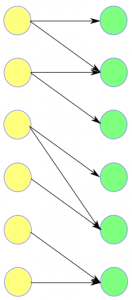
The training data is given as pairs of sets that correspond to matching predicted spectra and mass spectra. These sets can be represented in binary form. The goal is to learn the structure and the parameters of a bipartite graphical model from the training data (Figure 14).
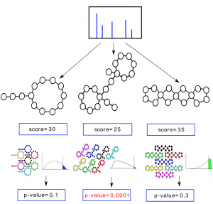
Figure 13. P-value of a match between metabolomics and metagenomics data is defined as the portion of randomly generated data with scores exceeding match score.
{7, 14, 25, 28} & {8, 15, 17, 26}
{3, 12, 18, 21 , 22} & {4, 19, 22, 23}
…
(a)
[0,0,0,0,0,0,1,0,0,0,0,0,0,1,0,…] & [0,0,0,0,0,0,0,1,0,0,0,0,0,0,0,1,…]
[0,0,1,0,0,0,0,0,0,0,0,1,0,0,0,…] & [0,0,0,1,0,0,0,0,0,0,0,0,0,0,0,0,…]
…
(b)
(c)
Figure 14. (a) The training data is given as pairs of sets that correspond to matching predicted spectra and mass spectra, respectively. (b) These sets can be represented in binary form (c) The goal is to learn the structure and the parameters of the bipartite graphical model that describes the dependencies between the predicted spectra and the mass spectra.
Open Problems: Automated hypothesis generation
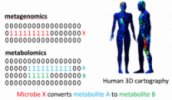
In recent years, researchers have developed large scale mass spectrometry and metagenomics data from environmental and host-oriented samples. One example is a 3D Cartography of human skin, where paired data are available from different parts of skin. Metagenomics tells us about what microbes are living on human skin, and metabolomics tells us about the chemicals they produce.
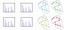
This pattern of co-occurrence of metabolomics and metagenomics features can be used for generating hypotheses about the relationships between microbes and chemicals. For example, if a metabolomics feature corresponding to chemical Y is present only at the intersection of occurrence patterns of a metabolomics feature corresponding to chemical X, and a metagenomics feature corresponding to microbe A, then one can hypothesize that microbe A might convert chemical X to chemical Y (Figure 15). The statistical significance of such hypotheses should be computed to avoid false hypotheses generation.
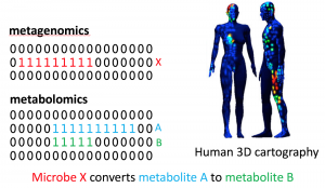
Figure 15. Automated hypotheses generation.
